Introduction to ascotraceR
ascotraceR is an R package of the ‘ascotraceR’ model developed to simulate the spread of Ascochyta blight in a chickpea field over a growing season. Parameters and variables used in the model were mostly derived from the literature and were subjected to validation in the field. The model uses daily weather data to simulate disease spread and a set of weather data is included with the package for demonstration purposes.
Getting started
Load the libraries.
Import the weather data using data that is included in the ascotraceR package.
# weather data
Billa_Billa <- fread(
  system.file(
    "extdata",
    "2020_Billa_Billa_weather_data_ozforecast.csv",
    package = "ascotraceR"
  )
)

# format time column
Billa_Billa[, local_time := dmy_hm(local_time)]

# specify the station coordinates of the Billa Billa weather station
Billa_Billa[, c("lat", "lon") := .(-28.1011505, 150.3307084)]

head(Billa_Billa)
## day local_time assessment_number mean_daily_temp wind_ km_h ws
## 1: 1 2020-06-04 00:00:00 NA 4.1 0.9 0.25
## 2: 1 2020-06-04 00:15:00 NA 3.9 0.6 0.17
## 3: 1 2020-06-04 00:30:00 NA 3.9 2.0 0.56
## 4: 1 2020-06-04 00:45:00 NA 4.3 1.2 0.33
## 5: 1 2020-06-04 01:00:00 NA 3.7 2.4 0.67
## 6: 1 2020-06-04 01:15:00 NA 3.5 1.3 0.36
## ws_sd wd wd_sd cummulative_rain_since_9am rain_mm wet_hours location
## 1: NA 215 NA 0 0 NA Billa_Billa
## 2: NA 215 NA 0 0 NA Billa_Billa
## 3: NA 215 NA 0 0 NA Billa_Billa
## 4: NA 215 NA 0 0 NA Billa_Billa
## 5: NA 215 NA 0 0 NA Billa_Billa
## 6: NA 215 NA 0 0 NA Billa_Billa
## lat lon
## 1: -28.10115 150.3307
## 2: -28.10115 150.3307
## 3: -28.10115 150.3307
## 4: -28.10115 150.3307
## 5: -28.10115 150.3307
## 6: -28.10115 150.3307Wrangle weather data
A function, format_weather(), is provided to convert raw weather data into the format appropriate for the model. It is mandatory to format weather data before running the model. Time zone can also be set manually using time_zone argument. If latitude and longitude are not supplied in the raw weather data, a separate CSV file listing latitude and longitude can be supplied to meet this requirement (see ?format_weather() for more details).
Billa_Billa <- format_weather(
  x = Billa_Billa,
  POSIXct_time = "local_time",
  temp = "mean_daily_temp",
  ws = "ws",
  wd_sd = "wd_sd",
  rain = "rain_mm",
  wd = "wd",
  station = "location",
  time_zone = "Australia/Brisbane",
  lon = "lon",
  lat = "lat"
)
Simulate Ascochyta blight spread
A function, trace_asco(), is provided to simulate the spread of Ascochyta blight in a chickpea field over a growing season. The inputs needed to run the function include weather data, paddock length and width, sowing and harvest dates, chickpea growing points replication rate, primary infection intensity, latent period, number of conidia produced per lesion and the location of primary infection foci (centre or random). The model output is a nested list with items for each day of the model run. See the help file for trace_asco() for more information.
# Predict Ascochyta blight spread for the year 2020 at Billa Billa
traced <- trace_asco(
  weather = Billa_Billa,
  paddock_length = 20,
  paddock_width = 20,
  initial_infection = "2020-07-17",
  sowing_date = "2020-06-04",
  harvest_date = "2020-10-27",
  time_zone = "Australia/Brisbane",
  seeding_rate = 40,
  gp_rr = 0.0065,
  spores_per_gp_per_wet_hour = 0.6,
  latent_period_cdd = 150,
  primary_inoculum_intensity = 100,
  primary_infection_foci = "centre"
)
Tidy up or summarise the model output
Functions tidy_trace() and summarise_trace() have been provided to tidy up and summarise the model output
Tidy up the model output
tidied <- tidy_trace(traced)
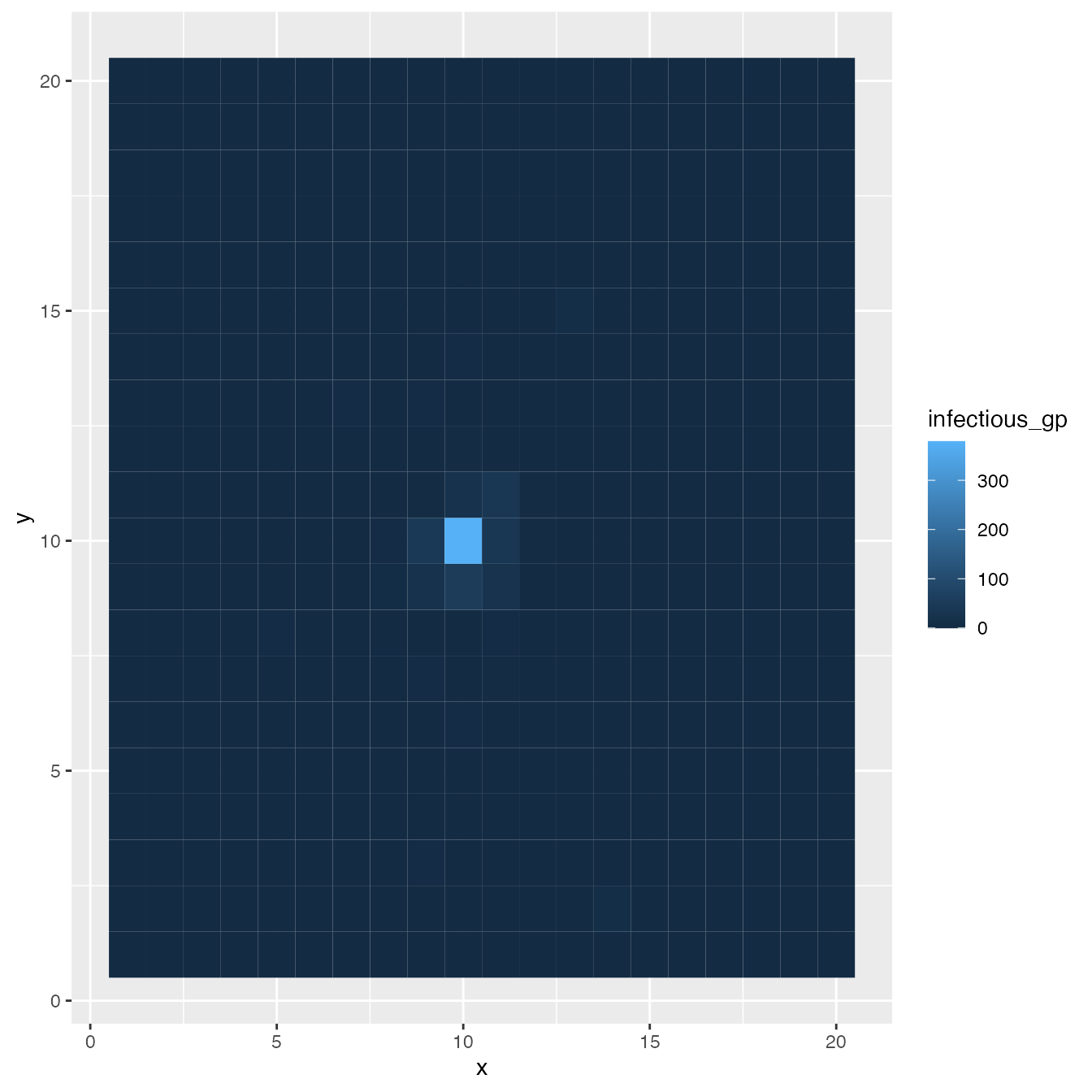
tidied## i_day i_date day x y new_gp susceptible_gp exposed_gp
## 1: 1 2020-06-04 156 1 1 40 40 0
## 2: 1 2020-06-04 156 1 2 40 40 0
## 3: 1 2020-06-04 156 1 3 40 40 0
## 4: 1 2020-06-04 156 1 4 40 40 0
## 5: 1 2020-06-04 156 1 5 40 40 0
## ---
## 58796: 147 2020-10-28 302 20 16 0 4981 0
## 58797: 147 2020-10-28 302 20 17 0 4981 0
## 58798: 147 2020-10-28 302 20 18 0 4981 0
## 58799: 147 2020-10-28 302 20 19 0 4981 0
## 58800: 147 2020-10-28 302 20 20 0 4981 0
## infectious_gp cdd cwh cr gp_standard
## 1: 0 0.000 0 0 40
## 2: 0 0.000 0 0 40
## 3: 0 0.000 0 0 40
## 4: 0 0.000 0 0 40
## 5: 0 0.000 0 0 40
## ---
## 58796: 0 2215.577 74 97 4981
## 58797: 0 2215.577 74 97 4981
## 58798: 0 2215.577 74 97 4981
## 58799: 0 2215.577 74 97 4981
## 58800: 0 2215.577 74 97 4981Summarise the model output
summarised <- summarise_trace(traced)
summarised
## i_day new_gp susceptible_gp exposed_gp infectious_gp i_date day
## 1: 1 16000 16000 0 0 2020-06-04 156
## 2: 2 1200 17200 0 0 2020-06-05 157
## 3: 3 1200 18400 0 0 2020-06-06 158
## 4: 4 1200 19600 0 0 2020-06-07 159
## 5: 5 1600 21200 0 0 2020-06-08 160
## ---
## 143: 143 0 1992398 11 781 2020-10-24 298
## 144: 144 1 1992399 11 781 2020-10-25 299
## 145: 145 0 1992399 11 781 2020-10-26 300
## 146: 146 1 1992395 6 786 2020-10-27 301
## 147: 147 1 1992396 6 786 2020-10-28 302
## cdd cwh cr gp_standard AUDPC
## 1: 0.00000 0 0.0 40 52542
## 2: 10.74583 0 0.0 43 52542
## 3: 22.84583 0 0.0 46 52542
## 4: 35.41042 0 0.0 49 52542
## 5: 49.38958 1 0.6 53 52542
## ---
## 143: 2133.81645 65 76.2 4981 52542
## 144: 2154.64770 73 94.4 4981 52542
## 145: 2176.49562 73 94.4 4981 52542
## 146: 2195.63104 73 94.4 4981 52542
## 147: 2215.57687 74 97.0 4981 52542