Fit GLMMs

Import data

# event data includes dates and time out and removed, exposure hours and 
# assessment date

event_data <- read_csv(system.file(
  "extdata",
  "exposure_events.csv",
  package = "rainy",
  mustWork = TRUE
)) %>%
  mutate(
    date_time_out = dmy_hm(date_time_out),
    date_time_removed = dmy_hm(date_time_removed),
    exposed = interval(date_time_out, date_time_removed)
  )

lesion_data <- read_csv(system.file(
  "extdata",
  "lesion_data.csv",
  package = "rainy",
  mustWork = TRUE
)) %>%
  pivot_longer(cols = plant_1:plant_3,
               names_to = "plant",
               values_to = "lesions") %>% 
  group_by(rainfall_event, pot) %>% 
  summarise(total_lesions = sum(lesions, na.rm = TRUE),
         mean_lesions = round(mean(lesions), 1))

Create object for analysis

Lastly we import the weather data and then:

filter for only the dates/times with plants deployed,
summarise by rainfall event, and then
join with the lesion data.

dat <- read_csv(system.file(
  "extdata",
  "weather_data.csv",
  package = "rainy",
  mustWork = TRUE
)) %>%
  mutate(
    Date_time = round_date(dmy_hms(paste(Date, Time)), "minute"),
    rain_duration = as.integer(`TOTAL Rain Gauge mm` > 0),
    rainfall_event = case_when(
      Date_time %within% event_data[1, "exposed"] ~ 1,
      Date_time %within% event_data[2, "exposed"] ~ 2,
      Date_time %within% event_data[3, "exposed"] ~ 3,
      Date_time %within% event_data[4, "exposed"] ~ 4,
      Date_time %within% event_data[5, "exposed"] ~ 5,
      Date_time %within% event_data[6, "exposed"] ~ 6,
      Date_time %within% event_data[7, "exposed"] ~ 7
    )
  ) %>%
  filter(
    Date_time %within% event_data[1, "exposed"] |
      Date_time %within% event_data[2, "exposed"] |
      Date_time %within% event_data[3, "exposed"] |
      Date_time %within% event_data[4, "exposed"] |
      Date_time %within% event_data[5, "exposed"] |
      Date_time %within% event_data[6, "exposed"] |
      Date_time %within% event_data[7, "exposed"]
  ) %>%
  group_by(rainfall_event) %>%
  summarise(
    wind_direction = round(circular.averaging(`AVERAGE Wind Direction Degs`), 1),
    total_rain = sum(`TOTAL Rain Gauge mm`),
    rain_duration = round(sum(rain_duration / 6), 1),
    temp = round(mean(`AVERAGE Air Temperature DegC`), 1),
    relative_humidity = round(mean(`AVERAGE Relative Humidity %`), 1),
    wind_speed = round(mean(`AVERAGE Wind Speed km/h`) * 0.277778, 1) # convert to m/s
  ) %>%
  left_join(lesion_data, by = "rainfall_event") %>%
  mutate(rainfall_event = as.factor(rainfall_event))

Check the data.

kableExtra::kable(dat,
      format = "html",
      table.attr = "class='table table-hover'")

rainfall_event	wind_direction	total_rain	rain_duration	temp	relative_humidity	wind_speed	pot	total_lesions	mean_lesions
1	93.7	1.4	0.8	19.6	89.6	4.2	1	0	0.0
1	93.7	1.4	0.8	19.6	89.6	4.2	2	1	0.3
1	93.7	1.4	0.8	19.6	89.6	4.2	3	0	0.0
1	93.7	1.4	0.8	19.6	89.6	4.2	4	1	0.3
1	93.7	1.4	0.8	19.6	89.6	4.2	5	0	0.0
1	93.7	1.4	0.8	19.6	89.6	4.2	6	0	0.0
1	93.7	1.4	0.8	19.6	89.6	4.2	7	0	0.0
1	93.7	1.4	0.8	19.6	89.6	4.2	8	0	0.0
1	93.7	1.4	0.8	19.6	89.6	4.2	9	0	0.0
1	93.7	1.4	0.8	19.6	89.6	4.2	10	0	0.0
1	93.7	1.4	0.8	19.6	89.6	4.2	11	0	0.0
1	93.7	1.4	0.8	19.6	89.6	4.2	12	0	0.0
2	87.1	2.8	0.7	21.0	83.2	3.7	1	5	1.7
2	87.1	2.8	0.7	21.0	83.2	3.7	2	7	2.3
2	87.1	2.8	0.7	21.0	83.2	3.7	3	7	2.3
2	87.1	2.8	0.7	21.0	83.2	3.7	4	0	0.0
2	87.1	2.8	0.7	21.0	83.2	3.7	5	1	0.3
2	87.1	2.8	0.7	21.0	83.2	3.7	6	10	3.3
2	87.1	2.8	0.7	21.0	83.2	3.7	7	0	0.0
2	87.1	2.8	0.7	21.0	83.2	3.7	8	1	0.3
2	87.1	2.8	0.7	21.0	83.2	3.7	9	1	0.3
2	87.1	2.8	0.7	21.0	83.2	3.7	10	0	0.0
2	87.1	2.8	0.7	21.0	83.2	3.7	11	0	0.0
2	87.1	2.8	0.7	21.0	83.2	3.7	12	0	0.0
3	95.4	3.4	1.7	20.3	90.1	4.5	1	0	0.0
3	95.4	3.4	1.7	20.3	90.1	4.5	2	0	0.0
3	95.4	3.4	1.7	20.3	90.1	4.5	3	3	1.0
3	95.4	3.4	1.7	20.3	90.1	4.5	4	4	1.3
3	95.4	3.4	1.7	20.3	90.1	4.5	5	0	0.0
3	95.4	3.4	1.7	20.3	90.1	4.5	6	1	0.3
3	95.4	3.4	1.7	20.3	90.1	4.5	7	1	0.3
3	95.4	3.4	1.7	20.3	90.1	4.5	8	1	0.3
3	95.4	3.4	1.7	20.3	90.1	4.5	9	0	0.0
3	95.4	3.4	1.7	20.3	90.1	4.5	10	1	0.3
3	95.4	3.4	1.7	20.3	90.1	4.5	11	2	0.7
3	95.4	3.4	1.7	20.3	90.1	4.5	12	2	0.7
4	198.1	13.4	7.0	10.5	76.8	2.9	1	41	NA
4	198.1	13.4	7.0	10.5	76.8	2.9	2	58	NA
4	198.1	13.4	7.0	10.5	76.8	2.9	3	121	40.3
4	198.1	13.4	7.0	10.5	76.8	2.9	4	46	15.3
4	198.1	13.4	7.0	10.5	76.8	2.9	5	12	NA
4	198.1	13.4	7.0	10.5	76.8	2.9	6	15	NA
4	198.1	13.4	7.0	10.5	76.8	2.9	7	30	10.0
4	198.1	13.4	7.0	10.5	76.8	2.9	8	22	7.3
4	198.1	13.4	7.0	10.5	76.8	2.9	9	65	NA
4	198.1	13.4	7.0	10.5	76.8	2.9	10	48	16.0
4	198.1	13.4	7.0	10.5	76.8	2.9	11	67	NA
4	198.1	13.4	7.0	10.5	76.8	2.9	12	72	NA
5	236.3	13.4	3.3	10.6	82.9	3.7	1	55	18.3
5	236.3	13.4	3.3	10.6	82.9	3.7	2	41	13.7
5	236.3	13.4	3.3	10.6	82.9	3.7	3	83	27.7
5	236.3	13.4	3.3	10.6	82.9	3.7	4	17	5.7
5	236.3	13.4	3.3	10.6	82.9	3.7	5	29	9.7
5	236.3	13.4	3.3	10.6	82.9	3.7	6	41	13.7
5	236.3	13.4	3.3	10.6	82.9	3.7	7	75	25.0
5	236.3	13.4	3.3	10.6	82.9	3.7	8	15	5.0
5	236.3	13.4	3.3	10.6	82.9	3.7	9	20	6.7
5	236.3	13.4	3.3	10.6	82.9	3.7	10	51	17.0
5	236.3	13.4	3.3	10.6	82.9	3.7	11	72	24.0
5	236.3	13.4	3.3	10.6	82.9	3.7	12	69	23.0
6	249.3	11.8	2.7	10.3	83.0	3.9	1	6	2.0
6	249.3	11.8	2.7	10.3	83.0	3.9	2	12	4.0
6	249.3	11.8	2.7	10.3	83.0	3.9	3	0	0.0
6	249.3	11.8	2.7	10.3	83.0	3.9	4	0	0.0
6	249.3	11.8	2.7	10.3	83.0	3.9	5	0	0.0
6	249.3	11.8	2.7	10.3	83.0	3.9	6	6	2.0
6	249.3	11.8	2.7	10.3	83.0	3.9	7	39	13.0
6	249.3	11.8	2.7	10.3	83.0	3.9	8	1	0.3
6	249.3	11.8	2.7	10.3	83.0	3.9	9	17	5.7
6	249.3	11.8	2.7	10.3	83.0	3.9	10	0	0.0
6	249.3	11.8	2.7	10.3	83.0	3.9	11	0	0.0
6	249.3	11.8	2.7	10.3	83.0	3.9	12	0	0.0
7	83.1	1.4	0.7	21.2	70.3	4.6	1	0	0.0
7	83.1	1.4	0.7	21.2	70.3	4.6	2	0	0.0
7	83.1	1.4	0.7	21.2	70.3	4.6	3	0	0.0
7	83.1	1.4	0.7	21.2	70.3	4.6	4	0	0.0
7	83.1	1.4	0.7	21.2	70.3	4.6	5	0	0.0
7	83.1	1.4	0.7	21.2	70.3	4.6	6	0	0.0
7	83.1	1.4	0.7	21.2	70.3	4.6	7	5	1.7
7	83.1	1.4	0.7	21.2	70.3	4.6	8	0	0.0
7	83.1	1.4	0.7	21.2	70.3	4.6	9	0	0.0
7	83.1	1.4	0.7	21.2	70.3	4.6	10	0	0.0
7	83.1	1.4	0.7	21.2	70.3	4.6	11	0	0.0
7	83.1	1.4	0.7	21.2	70.3	4.6	12	0	0.0

Use set.seed() for reproducibility purposes

set.seed(42)

Model_1 (All variables)

Include all variables with rainfall event as a random effect.

mod1 <-
  glmmTMB(
    total_lesions ~ total_rain +
      rain_duration +
      relative_humidity +
      temp +
      wind_speed +
      wind_direction +
      (1 | rainfall_event),
    family = nbinom1,
    data = dat
  )

## Warning in (function (start, objective, gradient = NULL, hessian = NULL, : NA/
## NaN function evaluation

summary(mod1)

##  Family: nbinom1  ( log )
## Formula:          
## total_lesions ~ total_rain + rain_duration + relative_humidity +  
##     temp + wind_speed + wind_direction + (1 | rainfall_event)
## Data: dat
## 
##      AIC      BIC   logLik deviance df.resid 
##    426.0    447.9   -204.0    408.0       75 
## 
## Random effects:
## 
## Conditional model:
##  Groups         Name        Variance  Std.Dev. 
##  rainfall_event (Intercept) 5.547e-18 2.355e-09
## Number of obs: 84, groups:  rainfall_event, 7
## 
## Dispersion parameter for nbinom1 family (): 12.4 
## 
## Conditional model:
##                    Estimate Std. Error z value Pr(>|z|)
## (Intercept)        5.790966        NaN     NaN      NaN
## total_rain         1.221316        NaN     NaN      NaN
## rain_duration     -0.694841        NaN     NaN      NaN
## relative_humidity  0.055962        NaN     NaN      NaN
## temp              -0.257993        NaN     NaN      NaN
## wind_speed        -0.009763        NaN     NaN      NaN
## wind_direction    -0.075632        NaN     NaN      NaN

The model summary suggest that there are not enough degrees of freedom to fit a complicated model. We can drop relative humidity and temperature because we directly transferred plants to a controlled environment with 20 degree Celsius temperature and 100 % RH

Model_2

Drop relative humidity and temperature

mod2 <-
  glmmTMB(
    total_lesions ~  total_rain +
      rain_duration +
      wind_speed +
      wind_direction + (1 | rainfall_event),
    family = nbinom1,
    data = dat
  )

## Warning in (function (start, objective, gradient = NULL, hessian = NULL, : NA/
## NaN function evaluation

summary(mod2)

##  Family: nbinom1  ( log )
## Formula:          
## total_lesions ~ total_rain + rain_duration + wind_speed + wind_direction +  
##     (1 | rainfall_event)
## Data: dat
## 
##      AIC      BIC   logLik deviance df.resid 
##    423.7    440.8   -204.9    409.7       77 
## 
## Random effects:
## 
## Conditional model:
##  Groups         Name        Variance  Std.Dev. 
##  rainfall_event (Intercept) 5.684e-10 2.384e-05
## Number of obs: 84, groups:  rainfall_event, 7
## 
## Dispersion parameter for nbinom1 family (): 12.4 
## 
## Conditional model:
##                Estimate Std. Error z value Pr(>|z|)    
## (Intercept)     2.87153    2.17801   1.318  0.18736    
## total_rain      1.25112    0.25352   4.935 8.01e-07 ***
## rain_duration  -0.58801    0.17224  -3.414  0.00064 ***
## wind_speed      0.21327    0.53217   0.401  0.68860    
## wind_direction -0.06191    0.01487  -4.164 3.13e-05 ***
## ---
## Signif. codes:  0 '***' 0.001 '**' 0.01 '*' 0.05 '.' 0.1 ' ' 1

We can see that model has been successful converged. But getting a warning message

Model_3

Remove wind speed as it is not significant

mod3 <-
  glmmTMB(
    total_lesions ~  total_rain +
      rain_duration +
      wind_direction + (1 | rainfall_event),
    family = nbinom1,
    data = dat
  )

## Warning in (function (start, objective, gradient = NULL, hessian = NULL, : NA/
## NaN function evaluation

summary(mod3)

##  Family: nbinom1  ( log )
## Formula:          
## total_lesions ~ total_rain + rain_duration + wind_direction +  
##     (1 | rainfall_event)
## Data: dat
## 
##      AIC      BIC   logLik deviance df.resid 
##    421.9    436.5   -205.0    409.9       78 
## 
## Random effects:
## 
## Conditional model:
##  Groups         Name        Variance  Std.Dev. 
##  rainfall_event (Intercept) 4.131e-10 2.032e-05
## Number of obs: 84, groups:  rainfall_event, 7
## 
## Dispersion parameter for nbinom1 family (): 12.4 
## 
## Conditional model:
##                Estimate Std. Error z value Pr(>|z|)    
## (Intercept)     3.69821    0.77355   4.781 1.75e-06 ***
## total_rain      1.22252    0.23032   5.308 1.11e-07 ***
## rain_duration  -0.61273    0.16398  -3.737 0.000186 ***
## wind_direction -0.06013    0.01342  -4.481 7.42e-06 ***
## ---
## Signif. codes:  0 '***' 0.001 '**' 0.01 '*' 0.05 '.' 0.1 ' ' 1

Again getting a warning message. And the negative impact of increasing rain duration and wind direction does not make any biological sense

Model_4

Replace wind direction with wind speed if the warning message could be removed

mod4 <-
  glmmTMB(
    total_lesions ~
      total_rain +
      rain_duration +
      wind_speed +
      (1 | rainfall_event),
    family = nbinom1,
    data = dat
  )

summary(mod4)

##  Family: nbinom1  ( log )
## Formula:          
## total_lesions ~ total_rain + rain_duration + wind_speed + (1 |  
##     rainfall_event)
## Data: dat
## 
##      AIC      BIC   logLik deviance df.resid 
##    437.6    452.2   -212.8    425.6       78 
## 
## Random effects:
## 
## Conditional model:
##  Groups         Name        Variance Std.Dev.
##  rainfall_event (Intercept) 0.3794   0.616   
## Number of obs: 84, groups:  rainfall_event, 7
## 
## Dispersion parameter for nbinom1 family (): 13.6 
## 
## Conditional model:
##               Estimate Std. Error z value Pr(>|z|)  
## (Intercept)    3.77220    4.27811   0.882   0.3779  
## total_rain     0.17733    0.08854   2.003   0.0452 *
## rain_duration  0.06054    0.27810   0.218   0.8277  
## wind_speed    -0.88854    0.96164  -0.924   0.3555  
## ---
## Signif. codes:  0 '***' 0.001 '**' 0.01 '*' 0.05 '.' 0.1 ' ' 1

The warning message has gone now. The reason is that wind direction did not vary much during different rainfall events, whereas wind speed varied. We can go with mod4.

Best fit model `mod4` diagnostics

Check over-dispersion

Check for over-dispersion using custom function created by Ben Bolker. Here is the link.

overdisp_fun <- function(model) {
  rdf <- df.residual(model)
  rp <- residuals(model, type = "pearson")
  Pearson.chisq <- sum(rp ^ 2)
  prat <- Pearson.chisq / rdf
  pval <- pchisq(Pearson.chisq, df = rdf, lower.tail = FALSE)
  c(
    chisq = Pearson.chisq,
    ratio = prat,
    rdf = rdf,
    p = pval
  )
}
overdisp_fun(mod4)

##      chisq      ratio        rdf          p 
## 48.8352552  0.6260930 78.0000000  0.9960638

The larger p value shows that there is no significant over-dispersion.

Simulate residuals

simulateResiduals(mod4, plot = T, quantreg = T)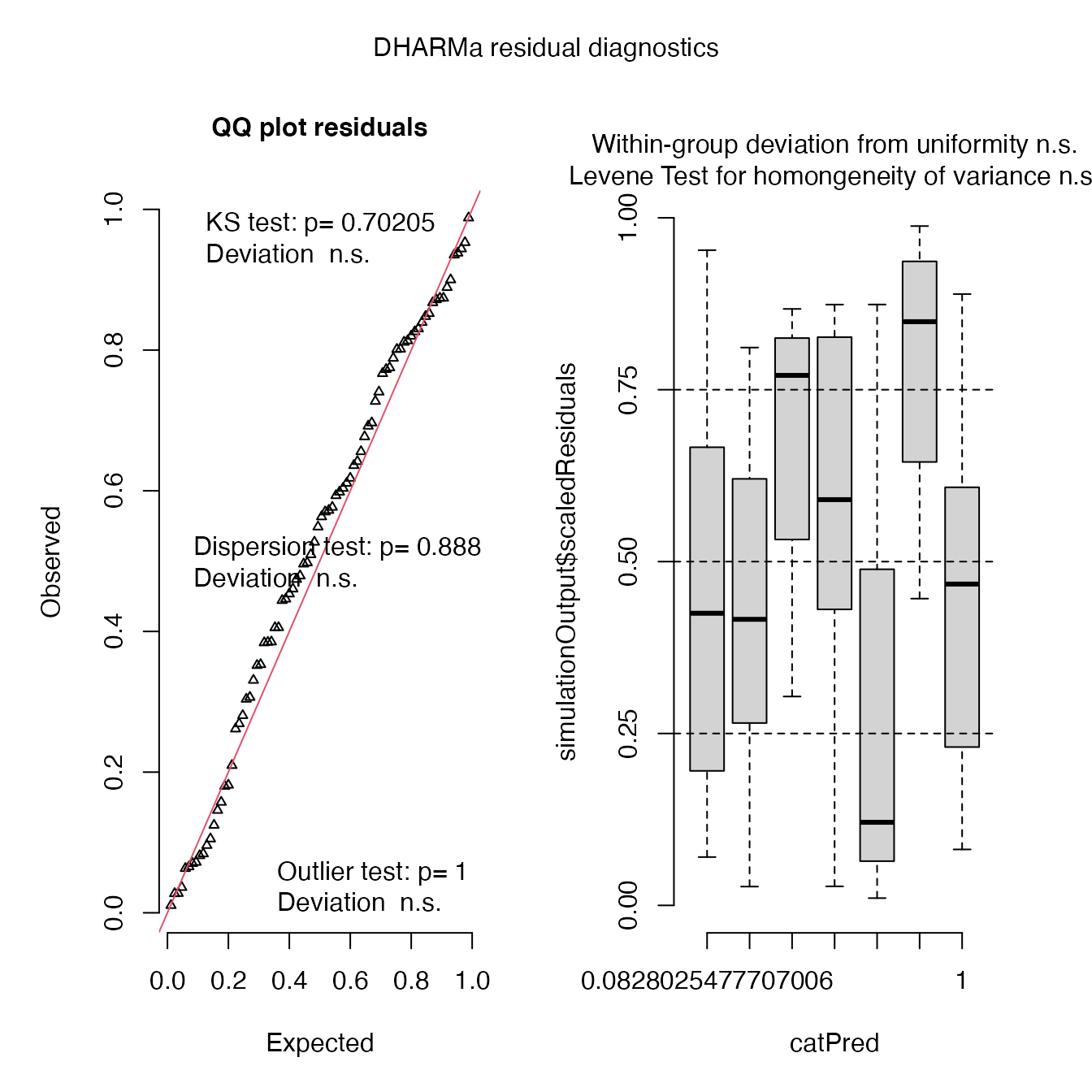

## Object of Class DHARMa with simulated residuals based on 250 simulations with refit = FALSE . See ?DHARMa::simulateResiduals for help. 
##  
## Scaled residual values: 0.02734823 0.8010679 0.3530158 0.8112905 0.2689484 0.6919764 0.3306609 0.4959772 0.1051955 0.2615026 0.4790774 0.5486829 0.8133635 0.8478606 0.8395191 0.3517644 0.6036274 0.8738153 0.02767958 0.6416688 ...

Very close observed and predicted values

Check zero-inflation

testZeroInflation(mod4)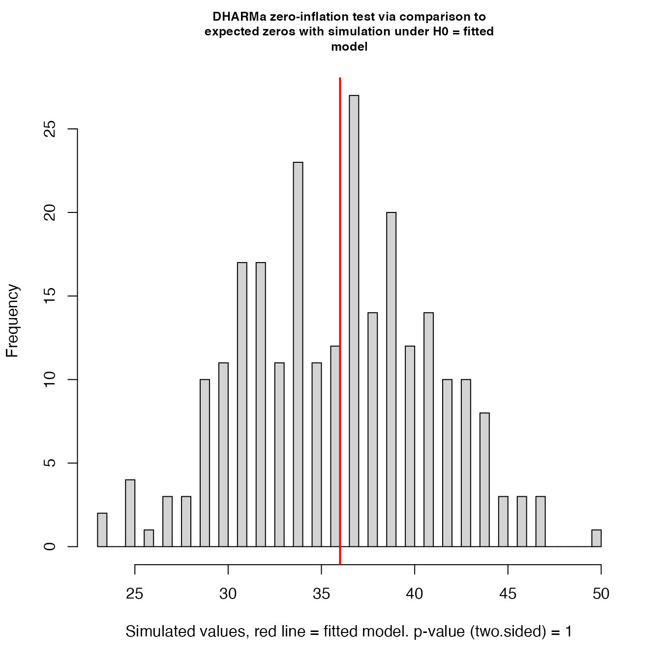

## 
##  DHARMa zero-inflation test via comparison to expected zeros with
##  simulation under H0 = fitted model
## 
## data:  simulationOutput
## ratioObsSim = 0.99767, p-value = 1
## alternative hypothesis: two.sided

No zero inflation detected

Check overall performance

performance::check_model(mod4, panel = FALSE)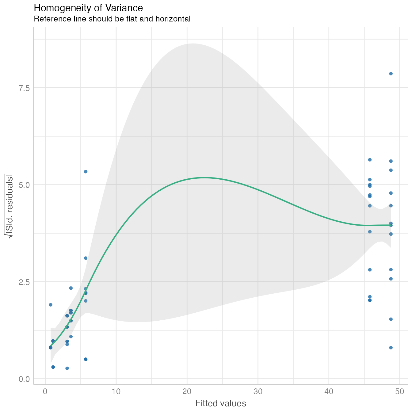

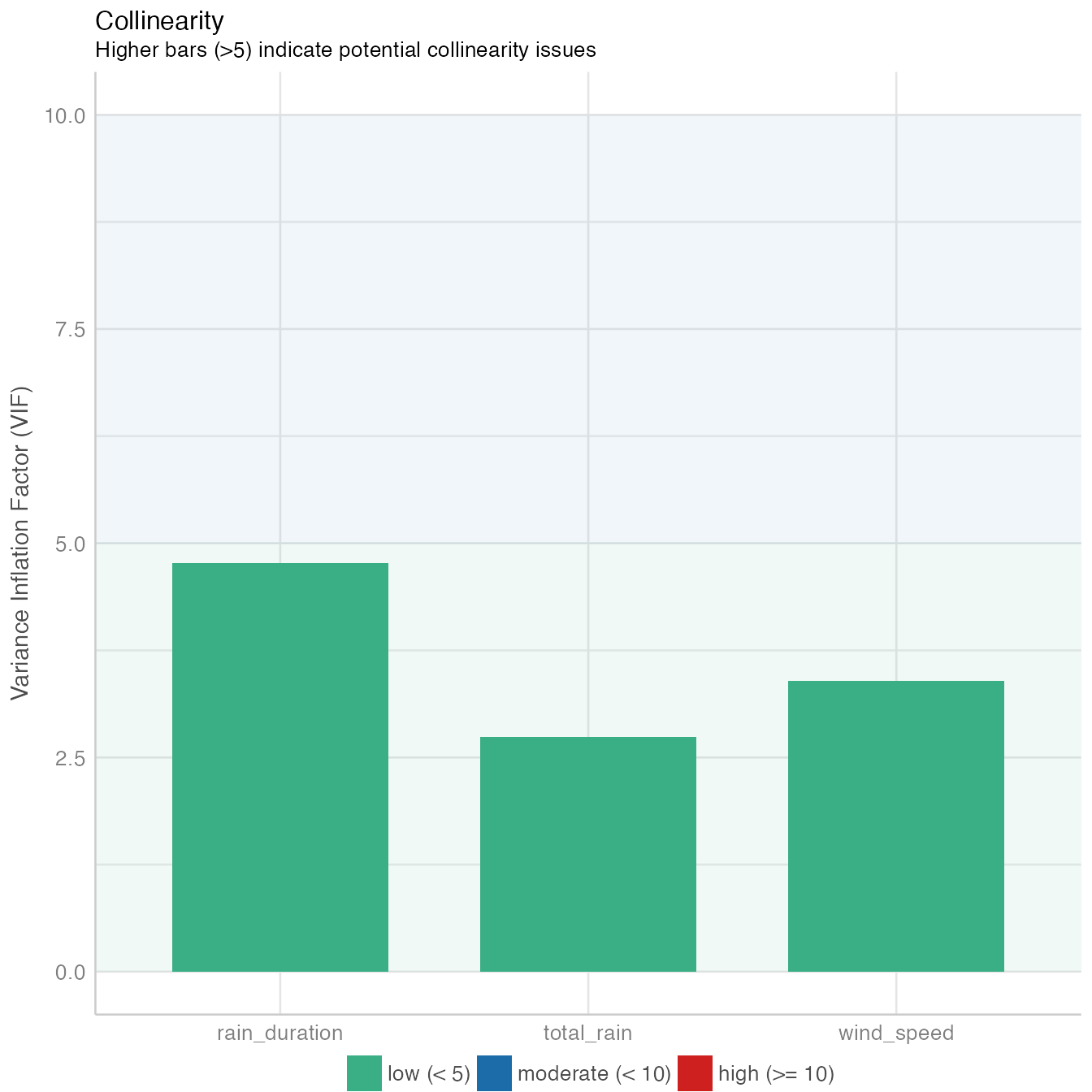
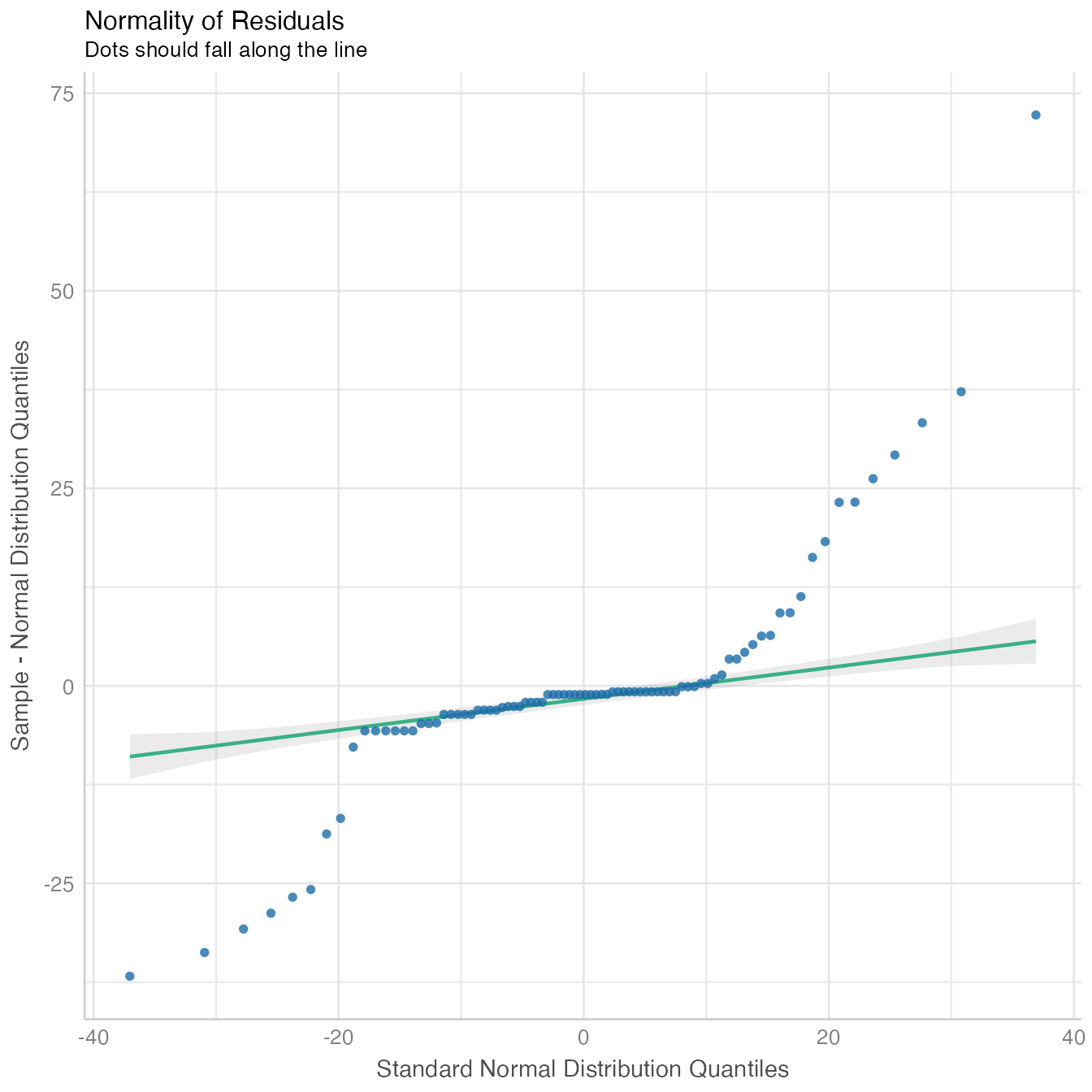
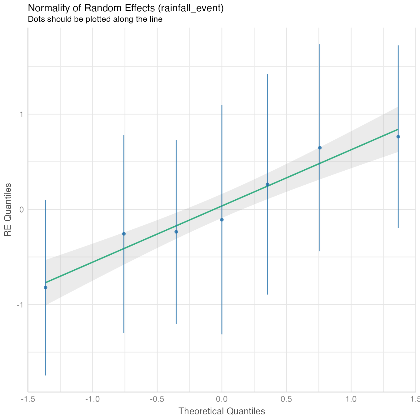
The model fit non-linear model data distribution assumption, close observed vs. fitted values and there is no significant collinearity between predictors.

Plot best fit model

f1 <-
  plot(ggpredict(mod4, "total_rain")) + 
  theme_pubclean(base_family = "Arial", base_size = 15)
f2 <-
  plot(ggpredict(mod4 , "rain_duration")) + 
  theme_pubclean(base_family = "Arial", base_size = 15)
f3 <-
  plot(ggpredict(mod4, "wind_speed")) + 
  theme_pubclean(base_family = "Arial", base_size = 15)
fig_4 <- grid.arrange(f1, f2, f3)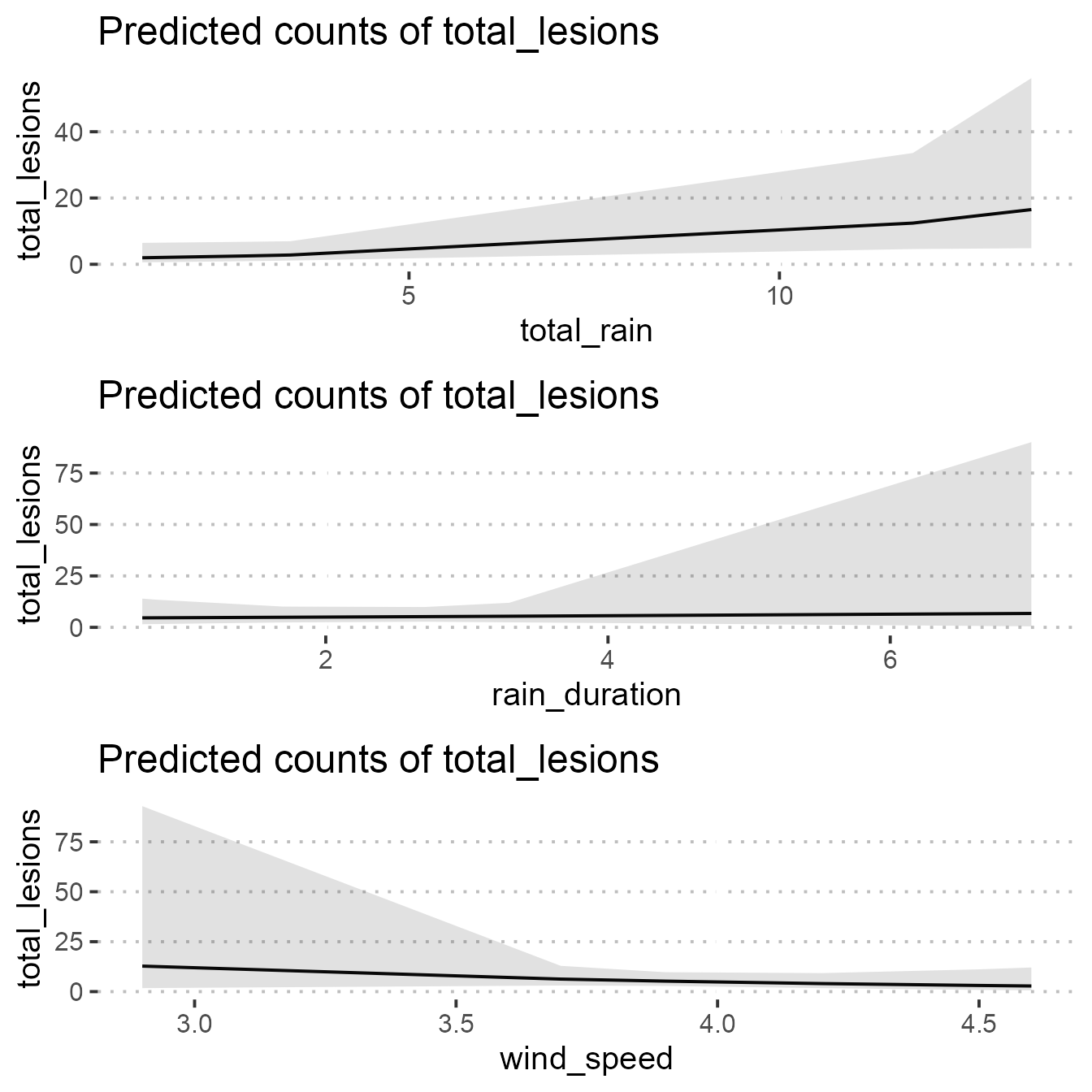

fig_4

## TableGrob (3 x 1) "arrange": 3 grobs
##   z     cells    name           grob
## 1 1 (1-1,1-1) arrange gtable[layout]
## 2 2 (2-2,1-1) arrange gtable[layout]
## 3 3 (3-3,1-1) arrange gtable[layout]

ggsave(
   here("man", "figures/fig_4.png"),
   plot = fig_4,
   width = 9,
   height = 9,
   units = "in",
   dpi = 600
)

ggsave(
   here("man", "figures/fig_4.eps"),
   plot = fig_4,
   width = 9,
   height = 9,
   units = "in",
   device =  cairo_ps
)

Colophon

sessionInfo()

## R version 4.1.0 (2021-05-18)
## Platform: x86_64-apple-darwin17.0 (64-bit)
## Running under: macOS Catalina 10.15.6
## 
## Matrix products: default
## BLAS:   /Library/Frameworks/R.framework/Versions/4.1/Resources/lib/libRblas.dylib
## LAPACK: /Library/Frameworks/R.framework/Versions/4.1/Resources/lib/libRlapack.dylib
## 
## locale:
## [1] en_AU.UTF-8/en_AU.UTF-8/en_AU.UTF-8/C/en_AU.UTF-8/en_AU.UTF-8
## 
## attached base packages:
## [1] stats     graphics  grDevices utils     datasets  methods   base     
## 
## other attached packages:
##  [1] ggpubr_0.4.0     lubridate_1.7.10 rainy_0.0.0.9000 gridExtra_2.3   
##  [5] here_1.0.1       ggeffects_1.1.0  DHARMa_0.4.2     glmmTMB_1.1.1   
##  [9] forcats_0.5.1    stringr_1.4.0    dplyr_1.0.7      purrr_0.3.4     
## [13] readr_1.4.0      tidyr_1.1.3      tibble_3.1.2     ggplot2_3.3.5   
## [17] tidyverse_1.3.1  readxl_1.3.1    
## 
## loaded via a namespace (and not attached):
##   [1] minqa_1.2.4         colorspace_2.0-2    ggsignif_0.6.2     
##   [4] ggridges_0.5.3      ellipsis_0.3.2      rio_0.5.27         
##   [7] sjlabelled_1.1.8    rprojroot_2.0.2     parameters_0.14.0  
##  [10] fs_1.5.0            rstudioapi_0.13     farver_2.1.0       
##  [13] fansi_0.5.0         xml2_1.3.2          codetools_0.2-18   
##  [16] splines_4.1.0       robustbase_0.93-8   cachem_1.0.5       
##  [19] knitr_1.33          jsonlite_1.7.2      nloptr_1.2.2.2     
##  [22] broom_0.7.8         dbplyr_2.1.1        effectsize_0.4.5   
##  [25] compiler_4.1.0      httr_1.4.2          backports_1.2.1    
##  [28] assertthat_0.2.1    Matrix_1.3-3        fastmap_1.1.0      
##  [31] cli_3.0.0           htmltools_0.5.1.1   tools_4.1.0        
##  [34] gtable_0.3.0        glue_1.4.2          Rcpp_1.0.6         
##  [37] carData_3.0-4       cellranger_1.1.0    jquerylib_0.1.4    
##  [40] pkgdown_1.6.1       vctrs_0.3.8         svglite_2.0.0      
##  [43] nlme_3.1-152        iterators_1.0.13    insight_0.14.2     
##  [46] xfun_0.24           openxlsx_4.2.4      lme4_1.1-27.1      
##  [49] rvest_1.0.0         lifecycle_1.0.0     rstatix_0.7.0      
##  [52] DEoptimR_1.0-9      MASS_7.3-54         scales_1.1.1       
##  [55] ragg_1.1.3          hms_1.1.0           qqplotr_0.0.5      
##  [58] TMB_1.7.20          yaml_2.2.1          curl_4.3.2         
##  [61] see_0.6.4           memoise_2.0.0       sass_0.4.0         
##  [64] stringi_1.6.2       bayestestR_0.10.0   highr_0.9          
##  [67] desc_1.3.0          gap_1.2.3-1         foreach_1.5.1      
##  [70] boot_1.3-28         zip_2.2.0           rlang_0.4.11       
##  [73] pkgconfig_2.0.3     systemfonts_1.0.2   evaluate_0.14      
##  [76] lattice_0.20-44     labeling_0.4.2      tidyselect_1.1.1   
##  [79] plyr_1.8.6          magrittr_2.0.1      R6_2.5.0           
##  [82] generics_0.1.0      DBI_1.1.1           mgcv_1.8-35        
##  [85] pillar_1.6.1        haven_2.4.1         foreign_0.8-81     
##  [88] withr_2.4.2         abind_1.4-5         performance_0.7.2  
##  [91] modelr_0.1.8        crayon_1.4.1        car_3.0-11         
##  [94] utf8_1.2.1          rmarkdown_2.9       grid_4.1.0         
##  [97] data.table_1.14.0   reprex_2.0.0        digest_0.6.27      
## [100] webshot_0.5.2       numDeriv_2016.8-1.1 textshaping_0.3.5  
## [103] munsell_0.5.0       viridisLite_0.4.0   kableExtra_1.3.4   
## [106] bslib_0.2.5.1

2021-07-14