Visualise data
Adam Sparks and Ihsan Khaliq
2021-07-16
a01_Visualise_Data.RmdLoad libraries
library("readxl")
library("cowplot")
library("ggplot2")
library("ggpubr")
library("grDevices")
library("dplyr")
library("lubridate")
library("clifro")
library("viridis")
library("showtext")
library("readr")
library("here")
library("patchwork")
library("classInt")
library("extrafont")

extrafont::loadfonts()
Import data
dat <-
   read_excel(
      system.file("extdata", "SpatioTemporalSpreadData_N.xlsx",
                  package = "spatiotemporaldynamics"),
      sheet = 1
   )
Examine data
str(dat)## tibble [1,800 × 18] (S3: tbl_df/tbl/data.frame)
## $ location : chr [1:1800] "Billa Billa" "Billa Billa" "Billa Billa" "Billa Billa" ...
## $ assessment_date : POSIXct[1:1800], format: "2020-07-02" "2020-07-02" ...
## $ assessment_number: num [1:1800] 1 1 1 1 1 1 1 1 1 1 ...
## $ plot_number : num [1:1800] 1 1 1 1 1 1 1 1 1 1 ...
## $ distance : num [1:1800] 0 9 9 9 9 9 9 9 9 6 ...
## $ quadrat : chr [1:1800] "F" "N9" "NE9" "E9" ...
## $ direction : chr [1:1800] "All" "North" "NorthEast" "East" ...
## $ infected_plants : num [1:1800] 0 0 0 0 0 0 0 0 0 0 ...
## $ total_plants : num [1:1800] 36 48 27 57 53 41 39 31 36 54 ...
## $ incidence : num [1:1800] 0 0 0 0 0 0 0 0 0 0 ...
## $ min_temp : num [1:1800] 3.99 3.99 3.99 3.99 3.99 ...
## $ max_temp : num [1:1800] 20 20 20 20 20 ...
## $ avg_temp : num [1:1800] 12 12 12 12 12 ...
## $ avg_wind_speed : num [1:1800] 1.52 1.52 1.52 1.52 1.52 ...
## $ total_rain : num [1:1800] 1 1 1 1 1 1 1 1 1 1 ...
## $ min_rh : num [1:1800] 35.2 35.2 35.2 35.2 35.2 ...
## $ max_rh : num [1:1800] 82.7 82.7 82.7 82.7 82.7 ...
## $ avg_rh : num [1:1800] 58.9 58.9 58.9 58.9 58.9 ...Convert variables to their correct classes
cols_1 <-
   c(
      "location",
      "distance",
      "plot_number",
      "quadrat",
      "min_temp",
      "max_temp",
      "min_rh",
      "max_rh",
      "avg_wind_speed",
      "avg_rh",
      "avg_temp",
      "assessment_number",
      "total_rain"
   )
dat[cols_1] <- lapply(dat[cols_1], factor)

cols_2 <- c("infected_plants", "total_plants")
dat[cols_2] <- lapply(dat[cols_2], as.integer)
dat$assessment_date <- as.Date(dat$assessment_date)
Re-check class
sapply(dat, class)## location assessment_date assessment_number plot_number
## "factor" "Date" "factor" "factor"
## distance quadrat direction infected_plants
## "factor" "factor" "character" "integer"
## total_plants incidence min_temp max_temp
## "integer" "numeric" "factor" "factor"
## avg_temp avg_wind_speed total_rain min_rh
## "factor" "factor" "factor" "factor"
## max_rh avg_rh
## "factor" "factor"Kernel denisty plots
Kernel density plot to visualise data distribution as by distance & location
ggplot(dat, aes(infected_plants)) +
   geom_density() +
   facet_grid(distance ~ location, labeller = label_both) +
   theme_pubclean(base_family = "Arial Unicode MS")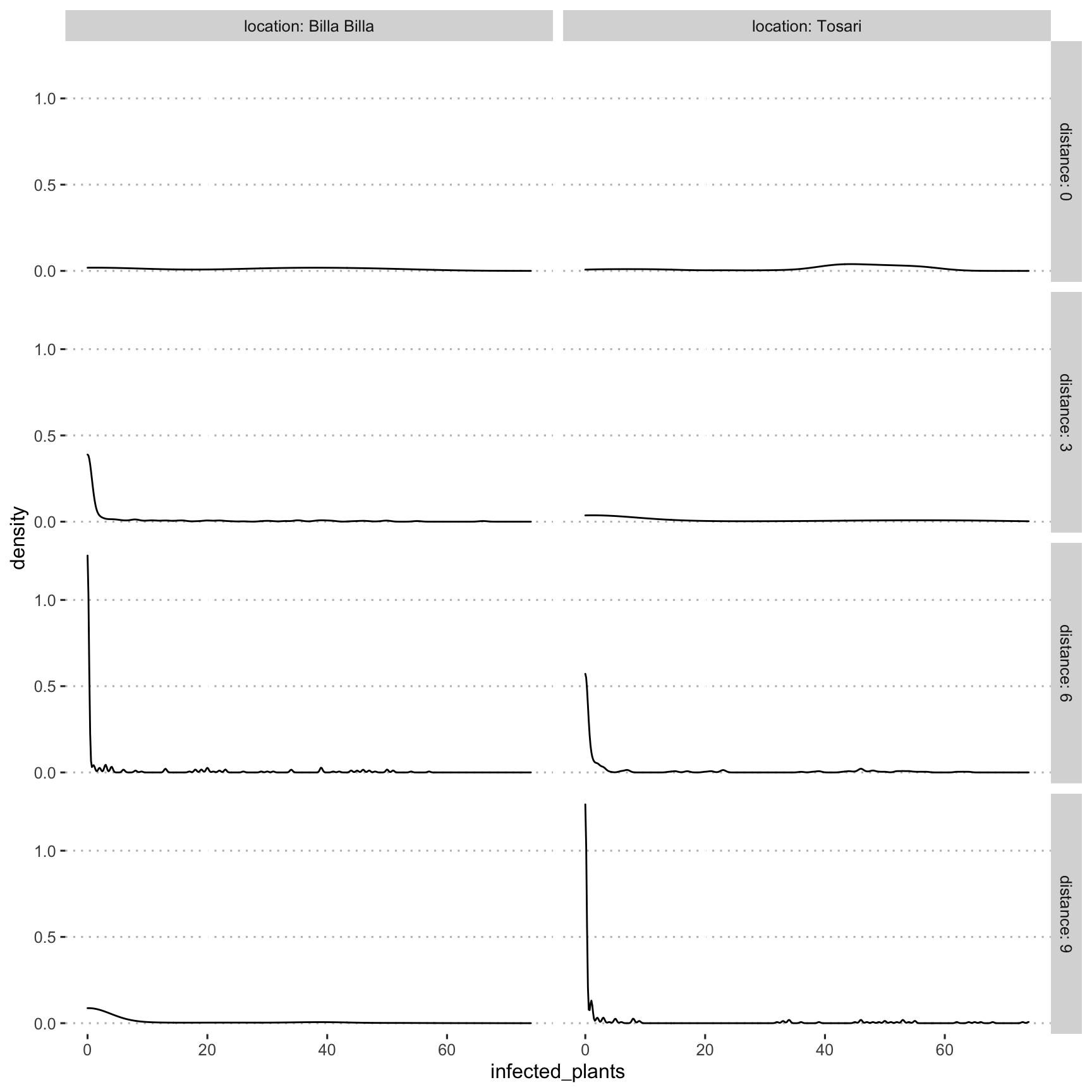
Kernel density plot to visualise overall data distribution
ggplot(dat, aes(x = infected_plants)) +
  geom_density(fill= "steelblue", alpha = 0.7) +
  geom_rug(alpha = 0.4) +
  xlab("Infected plants count")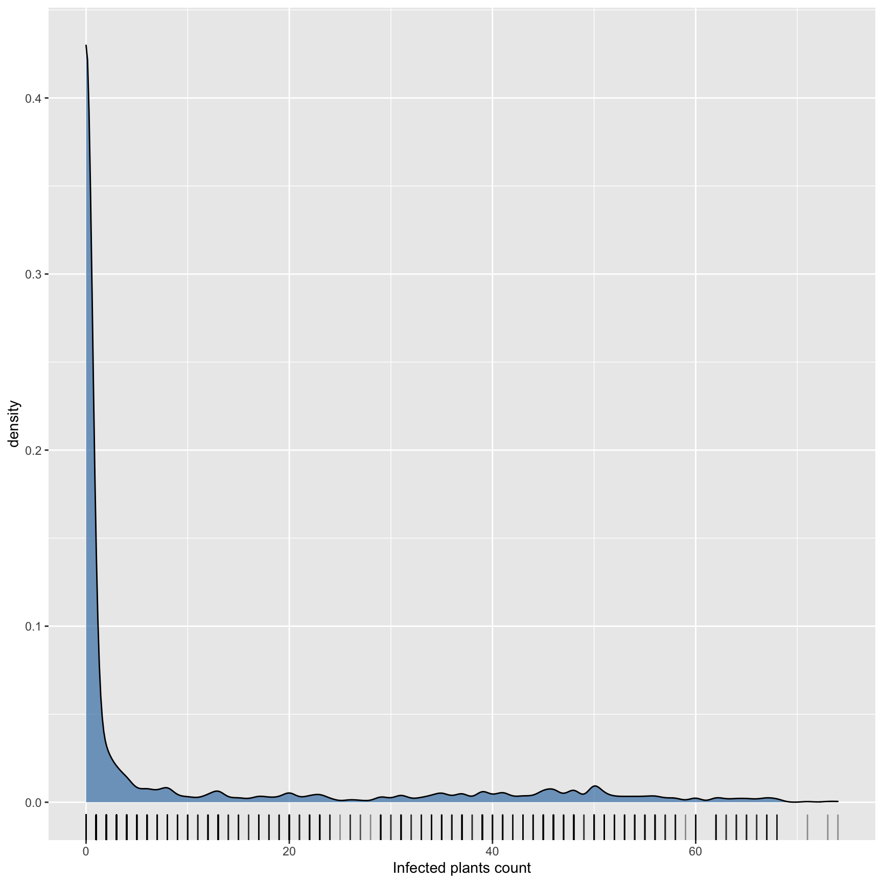
Line plot with median and max/min values
fig_1 <- ggplot(data = dat,
                mapping = aes(x = assessment_number, y = infected_plants)) +
   geom_pointrange(
      stat = "summary",
      fun.min = min,
      fun.max = max,
      fun = median
   ) +
   stat_summary(fun = median,
                geom = "line",
                aes(group = location)) +
   facet_grid(distance ~ location) +
   xlab("Assessment number") +
   ylab("Infected plants") +
   theme_pubclean(base_family = "Arial Unicode MS")

fig_1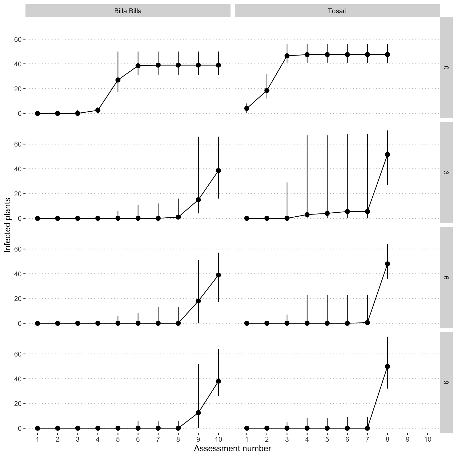
Wind rose
Import wind direction data and covert wind direction from text to degrees
# data munging
wind_direc_dat <-
   read_csv(
      system.file("extdata", "WindDirectionData.csv",
                  package = "spatiotemporaldynamics")
   ) %>%
   mutate(
      wind_direction_degrees = case_when(
         wind_direction == "N" ~ "0",
         wind_direction == "NbE" ~ "11.25",
         wind_direction == "NNE" ~ "22.5",
         wind_direction == "NEbN" ~ "33.75",
         wind_direction == "NE" ~ "45",
         wind_direction == "NEbE" ~ "56.25",
         wind_direction == "ENE" ~ "67.5",
         wind_direction == "EbN" ~ "73.5",
         wind_direction == "E" ~ "90",
         wind_direction == "EbS" ~ "101.2",
         wind_direction == "ESE" ~ "112.5",
         wind_direction == "SEbE" ~ "123.8",
         wind_direction == "SE" ~ "135.1",
         wind_direction == "SEbS" ~ "146.3",
         wind_direction == "SSE" ~ "157.6",
         wind_direction == "SbE" ~ "168.8",
         wind_direction == "S" ~ "180",
         wind_direction == "SbW" ~ "191.2",
         wind_direction == "SSW" ~ "202.5",
         wind_direction == "SWbS" ~ "213.8",
         wind_direction == "SW" ~ "225",
         wind_direction == "SWbW" ~ "236.2",
         wind_direction == "WSW" ~ "247.5",
         wind_direction == "WbS" ~ "258.8",
         wind_direction == "W" ~ "270",
         wind_direction == "WbN" ~ "281.2",
         wind_direction == "WNW" ~ "292.5",
         wind_direction == "NWbW" ~ "303.8",
         wind_direction == "NW" ~ "315",
         wind_direction == "NWbN" ~ "326.2",
         wind_direction == "NNW" ~ "337.5",
         wind_direction == "NbW" ~ "348.8",
         TRUE ~ wind_direction
      )
   ) %>%
   mutate(wind_direction_degrees = as.numeric(wind_direction_degrees)) %>%
   mutate(date = dmy(date))
##
## ── Column specification ────────────────────────────────────────────────────────
## cols(
## date = col_character(),
## location = col_character(),
## wind_direction = col_character()
## )Join wind speed and wind direction data
# Import wind speed data
wind_speed_dat <-
   read_csv(system.file("extdata", "WindSpeedData.csv",
                        package = "spatiotemporaldynamics")) %>%
   mutate(date = as_date(dmy_hm(date)))
##
## ── Column specification ────────────────────────────────────────────────────────
## cols(
## date = col_character(),
## location = col_character(),
## wind_speed = col_double()
## )
### Join wind speed and wind direction data
wind_dat <- left_join(wind_speed_dat, wind_direc_dat)
## Joining, by = c("date", "location")Plot windrose over chickpea growing season
fig_2 <-
   with(
      wind_dat,
      windrose(
         wind_speed,
         wind_direction_degrees,
         location,
         n_col = 2,
         legend_title = "Wind speed (m/s)"
      )
   )

fig_2 <-
   fig_2 +
   scale_fill_viridis_d(name = "Wind Speed (m/s)", direction = -1) +
   xlab("") +
   theme_pubclean(base_family = "Arial Unicode MS")

fig_2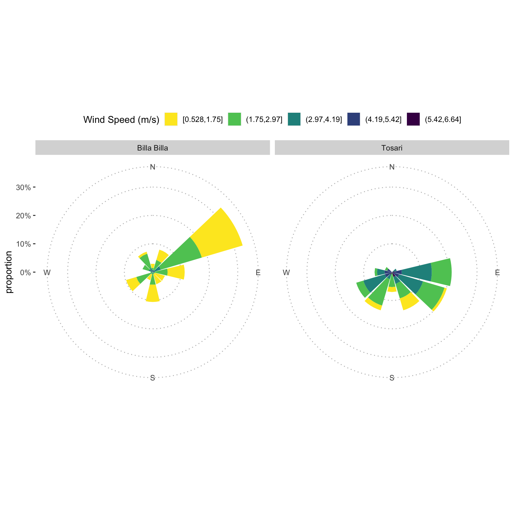
Data munging for ploting windrose by assessment number
# data munging
wind_dt <-
   wind_dat %>%
   mutate(
      assessment_number =
         case_when(
            date <= "2020-07-02" & location == "Billa Billa" ~ 1,
            date > "2020-07-02" &
               date <= "2020-07-16" & location == "Billa Billa" ~ 2,
            date > "2020-07-16" &
               date <= "2020-07-30" & location == "Billa Billa" ~ 3,
            date > "2020-07-30" &
               date <= "2020-08-13" & location == "Billa Billa" ~ 4,
            date > "2020-08-13" &
               date <= "2020-08-26" & location == "Billa Billa" ~ 5,
            date > "2020-08-26" &
               date <= "2020-09-10" & location == "Billa Billa" ~ 6,
            date > "2020-09-10" &
               date <= "2020-09-24" & location == "Billa Billa" ~ 7,
            date > "2020-09-24" &
               date <= "2020-10-08" & location == "Billa Billa" ~ 8,
            date > "2020-10-08" &
               date <= "2020-10-22" & location == "Billa Billa" ~ 9,
            date > "2020-10-22" &
               date <= "2020-10-27" &
               location == "Billa Billa" ~ 10,
            date <= "2020-07-30" & location == "Tosari" ~ 1,
            date > "2020-07-30" &
               date <= "2020-08-14" & location == "Tosari" ~ 2,
            date > "2020-08-14" &
               date <= "2020-08-27" & location == "Tosari" ~ 3,
            date > "2020-08-27" &
               date <= "2020-09-10" & location == "Tosari" ~ 4,
            date > "2020-09-10" &
               date <= "2020-09-25" & location == "Tosari" ~ 5,
            date > "2020-09-25" &
               date <= "2020-10-09" & location == "Tosari" ~ 6,
            date > "2020-10-09" &
               date <= "2020-10-23" & location == "Tosari" ~ 7,
            date > "2020-10-23" &
               date <= "2020-11-05" & location == "Tosari" ~ 8
         )
   ) %>%
   mutate(assessment_number  = as.factor(assessment_number))


Billa_Billa_wind_dt <- filter(wind_dt, location == "Billa Billa")
Tosari_wind_dt <- filter(wind_dt, location == "Tosari") %>%
   droplevels()
Plot windrose
# create breaks for the windroses
breaks <-
   classIntervals(wind_dat$wind_speed, n = 4, style = "jenks")

# Billa Billa windrose
fig_3.1 <-
   with(
      Billa_Billa_wind_dt,
      windrose(
         wind_speed,
         wind_direction_degrees,
         facet = assessment_number,
         n_col = 5,
         legend_title = "Wind speed (m/s)",
         speed_cuts = c(0, 1.4, 2.8, 4.2, 5.6, 7)
      )
   )

fig_3.1 <-
   fig_3.1 +
   scale_fill_viridis_d(name = "Wind Speed (m/s)",
                        direction = -1,
                        option = "cividis") +
   scale_y_continuous(name = "Proportion (%)",
                      labels = c(0, 10, 20, 30, 40, 50, 60)) +
   xlab("") +
   theme_pubclean(base_family = "Arial Unicode MS") +
   theme(
      axis.ticks.length = unit(0, "mm"),
      axis.line = element_blank(),
      panel.spacing.x = unit(0, "lines"),
      panel.spacing.y = unit(0, "lines"),
      plot.margin = margin(0, 0, 0, 0, "cm")
   )

# Tosari windrose
fig_3.2 <-
   with(
      Tosari_wind_dt,
      windrose(
         wind_speed,
         wind_direction_degrees,
         facet = assessment_number,
         n_col = 5,
         legend_title = "Wind speed (m/s)",
         speed_cuts = c(0, 1.4, 2.8, 4.2, 5.6, 7)
      )
   )

fig_3.2 <-
   fig_3.2 +
   scale_fill_viridis_d(name = "Wind Speed (m/s)",
                        direction = -1,
                        option = "cividis") +
   scale_y_continuous(name = "Proportion (%)",
                      labels = c(0, 10, 20, 30, 40, 50)) +
   xlab("") +
   theme_pubclean(base_family = "Arial Unicode MS") +
   theme(
      legend.position = "none",
      axis.ticks.length = unit(0, "mm"),
      axis.line = element_blank(),
      panel.spacing.x = unit(0, "lines"),
      panel.spacing.y = unit(0, "lines"),
      plot.margin = margin(0, 0, 0, 0, "cm")
   )

fig_3 <-
   fig_3.1 / fig_3.2

fig_3 <-
   fig_3 +
   plot_annotation(tag_levels = "A") &
   theme(plot.tag = element_text())

fig_3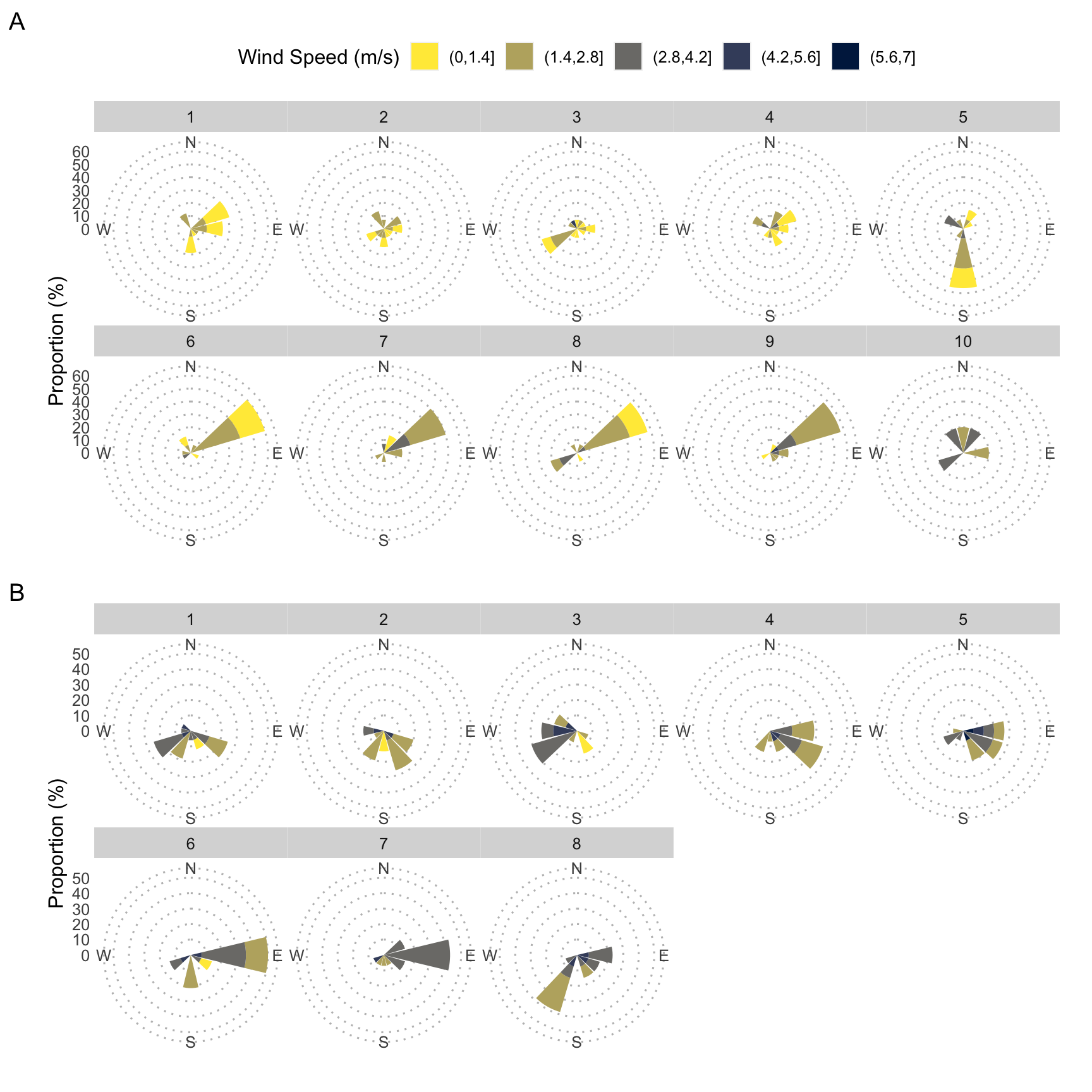
Colophon
## R version 4.1.0 (2021-05-18)
## Platform: x86_64-apple-darwin17.0 (64-bit)
## Running under: macOS Catalina 10.15.6
##
## Matrix products: default
## BLAS:   /Library/Frameworks/R.framework/Versions/4.1/Resources/lib/libRblas.dylib
## LAPACK: /Library/Frameworks/R.framework/Versions/4.1/Resources/lib/libRlapack.dylib
##
## locale:
## [1] en_AU.UTF-8/en_AU.UTF-8/en_AU.UTF-8/C/en_AU.UTF-8/en_AU.UTF-8
##
## attached base packages:
## [1] stats     graphics  grDevices utils     datasets  methods   base
##
## other attached packages:
##  [1] extrafont_0.17    classInt_0.4-3    patchwork_1.1.1   here_1.0.1
##  [5] readr_1.4.0       showtext_0.9-2    showtextdb_3.0    sysfonts_0.8.3
##  [9] viridis_0.6.1     viridisLite_0.4.0 clifro_3.2-5      lubridate_1.7.10
## [13] dplyr_1.0.7       ggpubr_0.4.0      ggplot2_3.3.5     cowplot_1.1.1
## [17] readxl_1.3.1
##
## loaded via a namespace (and not attached):
##  [1] fs_1.5.0           RColorBrewer_1.1-2 httr_1.4.2         rprojroot_2.0.2
##  [5] tools_4.1.0        backports_1.2.1    bslib_0.2.5.1      utf8_1.2.1
##  [9] R6_2.5.0           KernSmooth_2.23-20 DBI_1.1.1          colorspace_2.0-2
## [13] withr_2.4.2        tidyselect_1.1.1   gridExtra_2.3      curl_4.3.2
## [17] compiler_4.1.0     extrafontdb_1.0    cli_3.0.0          rvest_1.0.0
## [21] xml2_1.3.2         desc_1.3.0         labeling_0.4.2     sass_0.4.0
## [25] scales_1.1.1       proxy_0.4-26       pkgdown_1.6.1      stringr_1.4.0
## [29] digest_0.6.27      foreign_0.8-81     rmarkdown_2.9      rio_0.5.27
## [33] pkgconfig_2.0.3    htmltools_0.5.1.1  highr_0.9          fastmap_1.1.0
## [37] rlang_0.4.11       rstudioapi_0.13    farver_2.1.0       jquerylib_0.1.4
## [41] generics_0.1.0     jsonlite_1.7.2     zip_2.2.0          car_3.0-11
## [45] magrittr_2.0.1     Rcpp_1.0.7         munsell_0.5.0      fansi_0.5.0
## [49] abind_1.4-5        lifecycle_1.0.0    stringi_1.6.2      yaml_2.2.1
## [53] carData_3.0-4      plyr_1.8.6         grid_4.1.0         forcats_0.5.1
## [57] crayon_1.4.1       haven_2.4.1        hms_1.1.0          knitr_1.33
## [61] pillar_1.6.1       ggsignif_0.6.2     reshape2_1.4.4     glue_1.4.2
## [65] evaluate_0.14      data.table_1.14.0  vctrs_0.3.8        Rttf2pt1_1.3.8
## [69] cellranger_1.1.0   gtable_0.3.0       purrr_0.3.4        tidyr_1.1.3
## [73] assertthat_0.2.1   cachem_1.0.5       xfun_0.24          openxlsx_4.2.4
## [77] broom_0.7.8        e1071_1.7-7        rstatix_0.7.0      class_7.3-19
## [81] tibble_3.1.2       memoise_2.0.0      ellipsis_0.3.2